Excel 3D Reference is a short and flexible formula that lets you perform calculations by referencing the same cell or a range of cells on multiple sheets. The use of 3D formulas eliminates the need to reference each cell, making calculations easier. When you apply the 3D formula once, it will include data from sheets you add later.
This article will explore how consolidating data into one sheet can help reduce the time it takes to calculate data across multiple sheets. Managing large amounts of information within a single worksheet can be easy and efficient, leading to accurate results under minimum demands.
Different Approaches to Sum Data in Excel
In Excel, the traditional way to sum information across multiple sheets is to manually add up each cell using the Sum Function. In contrast, manually adding them can become increasingly problematic if you have a large dataset of monthly sales for an extended time.
This is also not a dynamic method, so you will have to change formulas again if you add an extra sheet. Let's quickly look at how the consolidation of data, across multiple sheets, into a single sheet with the help of Excel 3D Reference helps to quickly and precisely sum up the data.
Syntax of Excel 3D Reference
Take a look at the syntax of a 3D referencing formula that sums the values in Cells B4 for four sheets, named January, February, March, and April.
=SUM(January:April!B4)As shown above, there are two main elements in the Excel 3D Formula. The first one refers to the names of the first and last sheets separated by a semicolon. In the second part, the same cell or range of cells is referenced across all four sheets.
In this case, SUM is used. You can also use any other formula during the calculation. However, the syntax for 3D reference remains the same. To use Excel's 3D reference, the data must be consistent across the four sheets.
Excel 3D Reference Example
Now let's understand the rationale behind Excel 3D function. To assess this, let's put it into practice using a data set.
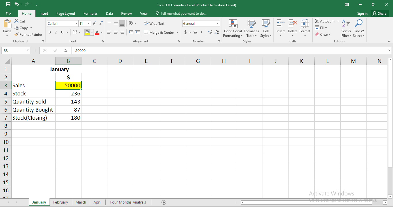
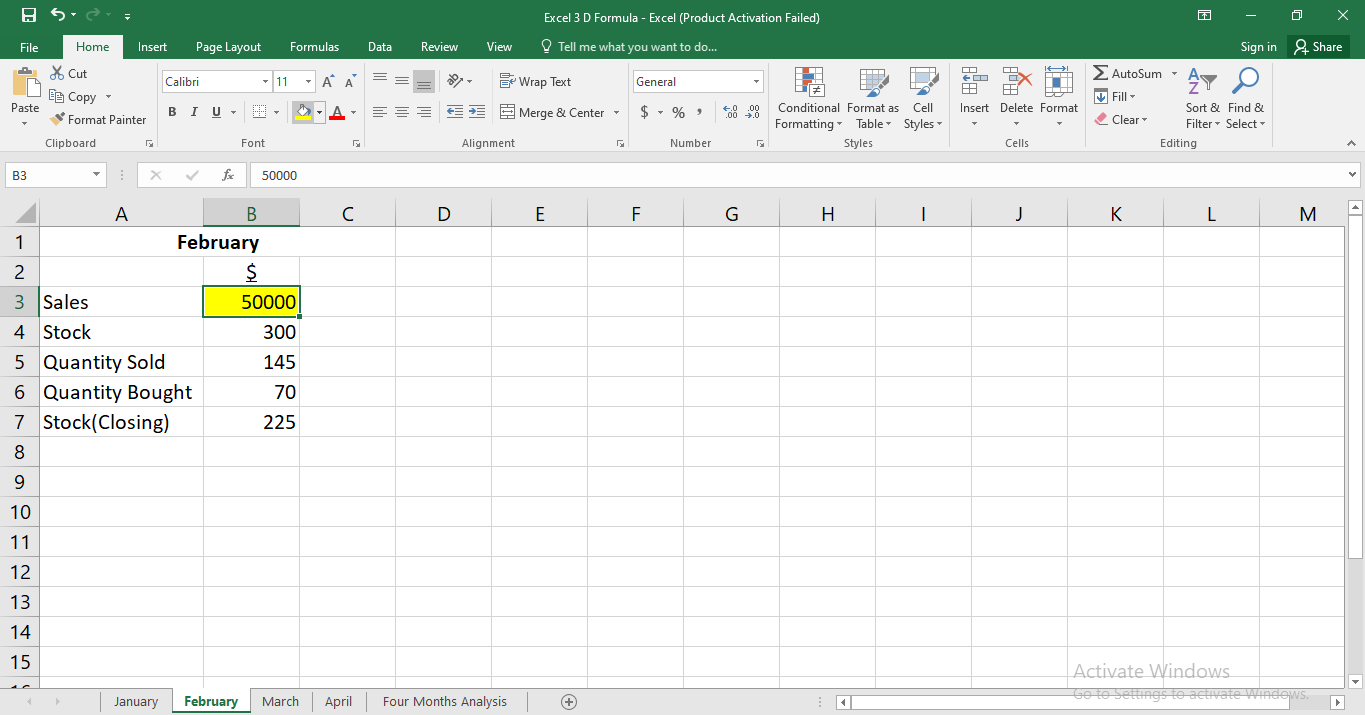
Take a look at the sample data that contains sales for the four months, stock number, stock sold, stock bought, and closing stock at the end of each month.
January Data:
February Data:
March Data:

April Data:
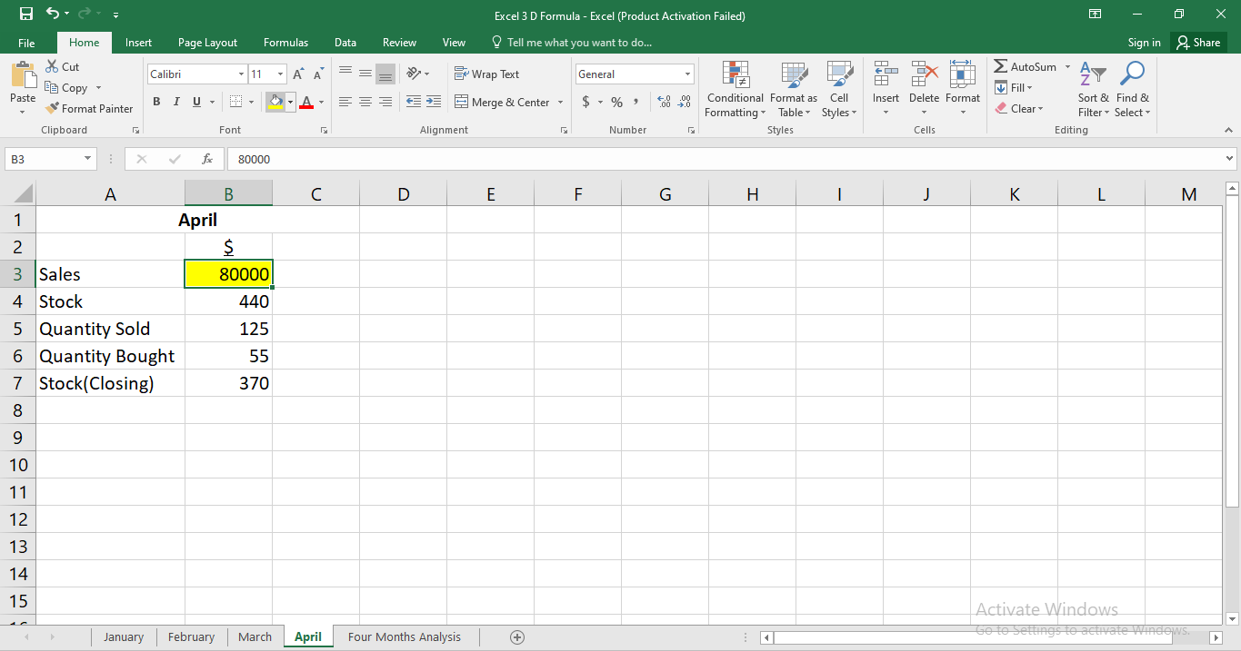
In the first step, assess the data available across four sheets to see if it is sequential. Only then can 3D references be implemented.
Related: How to Combine Multiple Data Sets in Microsoft Excel Using Power Query
Implementing the 3D Reference
To calculate the total sales for four months, select the cell where the figure will appear.
For this example, the sales value resides in cell B3 for all four sheets; the reference data across four sheets will be in the same cell. The range will appear from January to April because both are set names for starting and ending sheets, respectively.
1. Add cell B3 as a reference cell.
2. From January to April, choose the range to use.
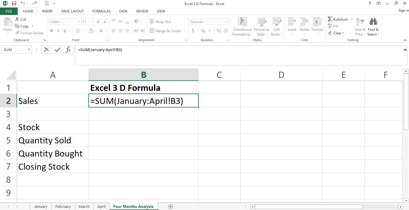
3. Press Enter to execute the formula.
To ensure that formula has been applied correctly, you can manually sum the values for a specific element in the data set. Once you know it's correct, you can expect the rest of the calculations to be correct as long as the values are consistent.
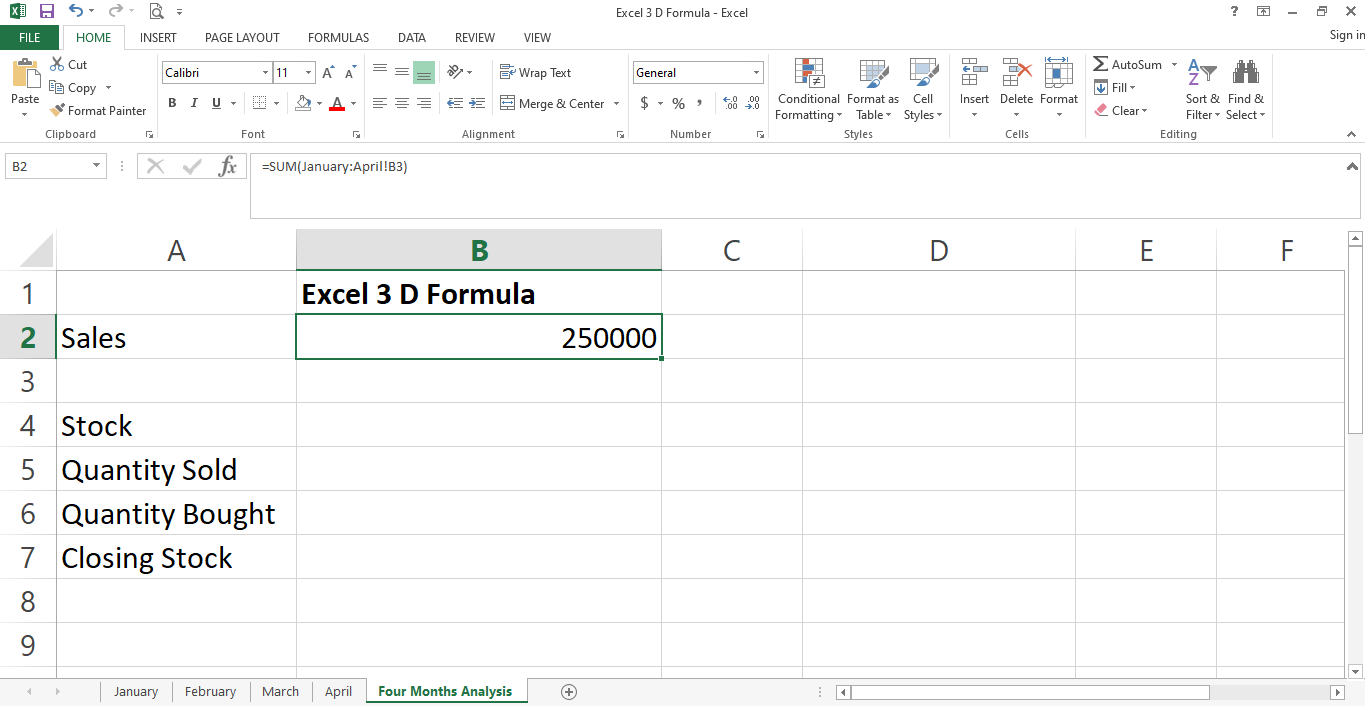
The same approach for calculating total sales value for four months applies to stock, stock bought, sold, and closing stock at the end of each month.
The range remains the same for four months, while the referenced cell will change according to their location in different sheets. Let's sum the Stock data for four months.
1. Add cell B4 as a reference cell.
2. Choose range as of January: April.
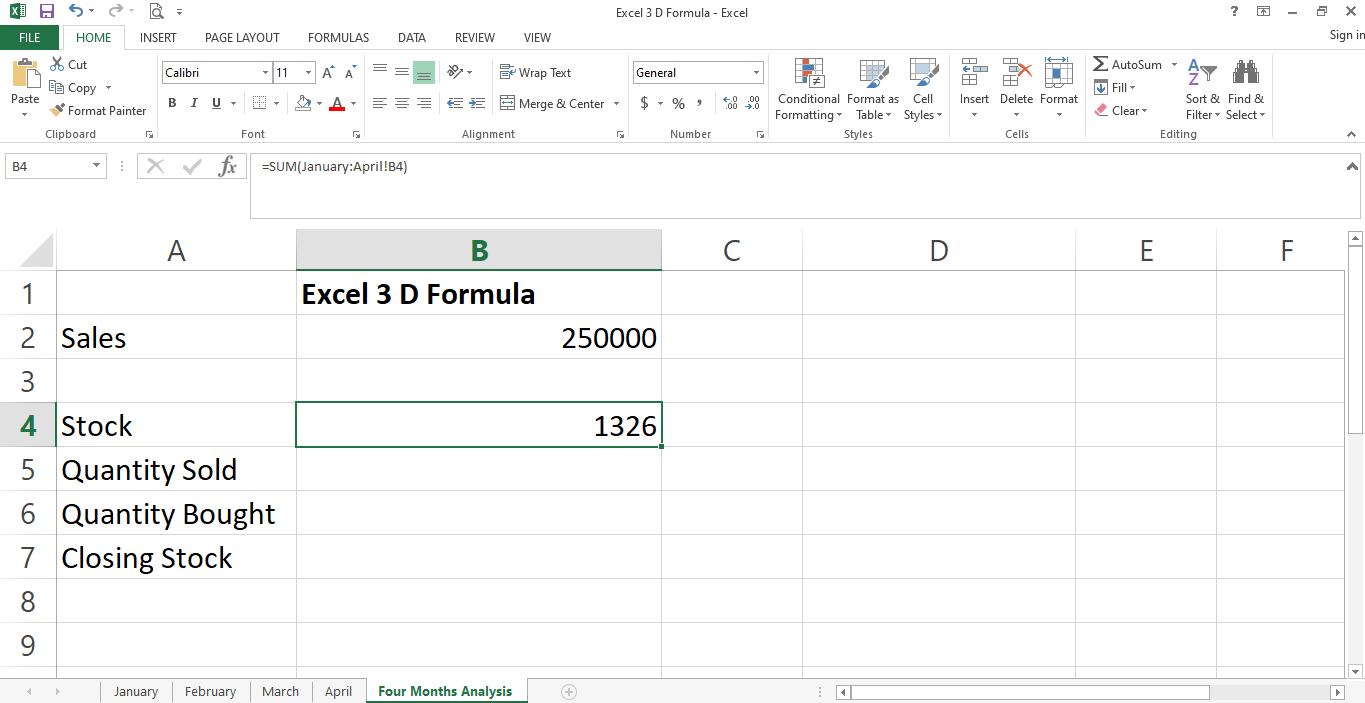
Drag it to implement the 3D sum formula for other cells in the row using the auto-fill sequence.
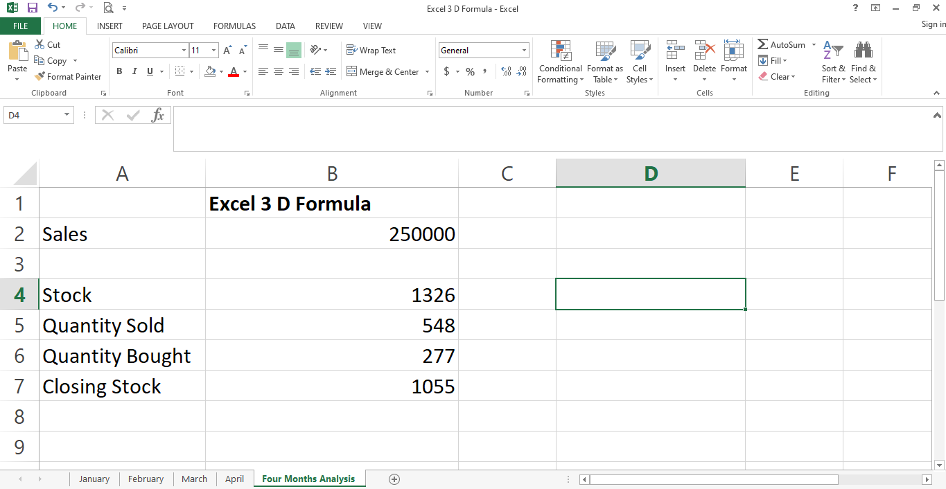
In the same way, you can apply 3D references to a range of cells on different worksheets. In this case, the selection of the sheets remains the same.
However, you need to choose the entire range instead of one cell as a reference. Also, ensure that the data is consistent across all sheets.
Adding New Sheet in Workbook
Excel 3D reference automatically updates data while adding one or more new sheets as long as those sheets fall between the ranges selected in the 3D formula. Let's see how it works.
As shown below, the total sales for four months are 250000 for the months January to April.

Let's add a new sheet containing the data for the mid-Feb month.
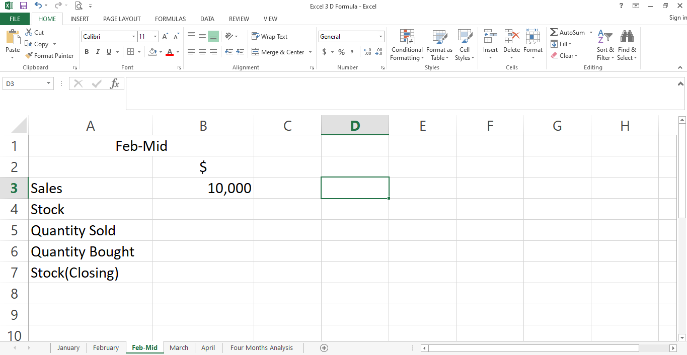
Incorporate the mid-Feb sheet's sales value. The data will automatically appear in the main sheet of the four-month analysis.
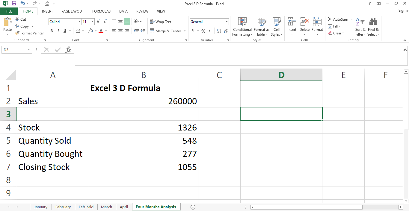
As shown above, the total sales for all months increase by an amount of 10,000. Thus, without altering the formula, the result has been updated automatically.
This flexibility comes in handy while tracking the sales record of the whole year across massive datasets. Let's add stock, quantity sold, the quantity bought, and ending stock data to the mid-Feb sheet.
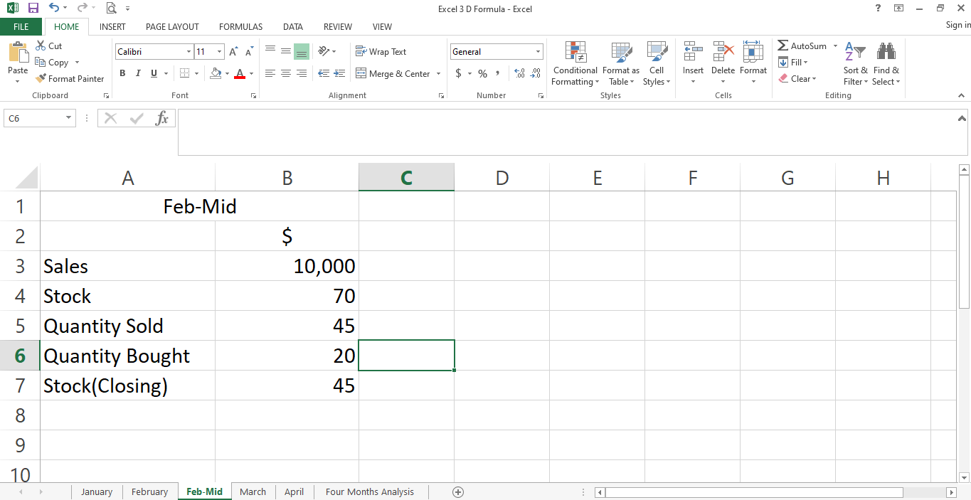
Take a look at how the above addition impacts the data in four months analysis sheet.
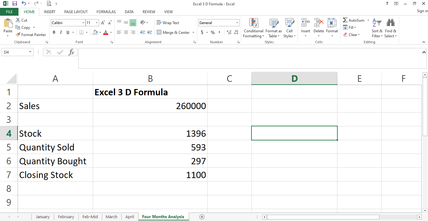
Therefore, the reference formula has successfully updated all of the data in the main sheet.
Related: How to Use Excel's Flash Fill and AutoFill to Automate Data Entry
Make Data Consistent to Apply 3D References
When you plan to consolidate data from multiple sheets into one, make sure it's consistent in cell number. If, for example, stock purchased is located in a certain cell on sheet 1, it is necessary to place it in the same cell on all the other sheets. Also, when adding a new sheet, enter data correctly across the cells.
Make Calculations Simpler With Excel 3D Referencing
Implementing 3D formulas may seem challenging to implement, but they are effortless to maintain once you execute them right. It lets you add new data every month without having to do the calculations from the start.
The 3D formula also eliminates the chances of duplication or omission of sales for any given month. This functionality will be most beneficial for accountants who update bundles of data every month.

